Predicting Undergraduate Dropout w/ Various ML models

Predicting Undergraduate Dropout

Introduction to the Problem

The United States has been grappling with a concerning issue of college dropouts for several years. According to recent data from ThinkImpact (2021), only 41% of students are able to graduate within four years without any delay. This educational failure is not only a major social issue that impacts the entire society, but it also results in a staggering annual loss of $3.8 billion.

On an individual level, individuals who have only completed high school are approximately three times more likely to live in poverty when compared to those who hold a bachelor’s degree (EDI, 2021). Societally, a lower level of education can have detrimental effects on economic growth, employment, and productivity. Hence, it is imperative to identify and address the problem of college dropouts to prevent or support students in need so that they can successfully navigate their way to graduation.

Interesting Aspects of the Problem

Previous analysis on the internet revealed several interesting aspects that can be used to identify students at higher risk of dropping out of college. Perhaps we can use these traits to predict students at higher risk, making academic/financial aids more accessible for them.

• 30% of College drop out in the first year
• 40% of College dropouts have parents who did not complete higher education
• only 8 to 10% of Foster kids graduate from college
• 51% of college dropouts drop out because of the lack of money.
• 5% of students 19 years or younger drop out.
• For students between the age of 20 and 23, 51% drop out.
• 31% of African American students, and 18% of Europian students drop out

Previous Works in the Field

In recent years, Learning Analytics (LA) and Educational Data Mining (EDM) have gained significant attention for their potential to improve education. These approaches have become popular due to several reasons.

1. Data-driven approaches have already shown effectiveness in business analytics, as demonstrated by Daradoumis et.al (2010). Therefore, it makes sense to employ these methods in the field of education as well.
2. The collection of refined educational data is relatively easy
3. universities are under constant pressure to reduce costs and increase income by reducing dropout rates and improving course quality.

While LA and EDM are similar in nature, LA deals more with applications, while EDM focuses more on techniques and methodologies. Until now, EDM methods have primarily focused on exploiting classical machine learning methods. However, with recent advancements in technology, it is worth exploring the application of neural networks to address the challenges in the education sector. By combining the strengths of LA and EDM and leveraging the power of neural networks, it may be possible to improve the quality of education and help reduce the dropout rates.

Our Interest

Currently, many studies in the field of Learning Analytics (LA) and Educational Data Mining (EDM) have utilized traditional Machine Learning (ML) methods. However, we want to explore the potentials of using Neural Networks, given the recent advancements in the field. Our objective is to predict undergraduate dropouts, which is a significant social issue as previously mentioned.

Our Dataset

The dataset we are working with originates from the Polytechnic Institute of Portalegre. It comprises 4424 records of students and contains 35 attributes, including enrollment status, demographics, socioeconomic status, and more.

Code Overview

1. Import & Initial Preprocessing
2. Initial Neural Network investigation
3. Finding Best Hyperparameter
4. Comparing with Non-Neural Network ML
5. Revisiting Preprocessing

Import & initial Preprocessing

Library Import

# Data Manipulation
import numpy as np
import pandas as pd

# Data Visualization
import seaborn as sns
import matplotlib.pyplot as plt


# NN ML
import torch
from torch.utils.data import Dataset, DataLoader
import torch.nn as nn

# non-NN ML
from sklearn import preprocessing
from sklearn.ensemble import RandomForestClassifier, ExtraTreesClassifier
from sklearn.svm import SVC
from sklearn.feature_selection import mutual_info_classif
from sklearn.model_selection import train_test_split, cross_val_score, GridSearchCV
from sklearn.neural_network import MLPClassifier
from sklearn.metrics import accuracy_score, confusion_matrix
from sklearn.tree import plot_tree

Data Import

data = pd.read_csv("dataset.csv",delimiter=';')
data.head()

	Marital status	Application mode	Application order	Course	Daytime/evening attendance	Previous qualification	Nacionality	Mother's qualification	Father's qualification	Mother's occupation	...	Curricular units 2nd sem (credited)	Curricular units 2nd sem (enrolled)	Curricular units 2nd sem (evaluations)	Curricular units 2nd sem (approved)	Curricular units 2nd sem (grade)	Curricular units 2nd sem (without evaluations)	Unemployment rate	Inflation rate	GDP	Target
0	1	8	5	2	1	1	1	13	10	6	...	0	0	0	0	0.000000	0	10.8	1.4	1.74	Dropout
1	1	6	1	11	1	1	1	1	3	4	...	0	6	6	6	13.666667	0	13.9	-0.3	0.79	Graduate
2	1	1	5	5	1	1	1	22	27	10	...	0	6	0	0	0.000000	0	10.8	1.4	1.74	Dropout
3	1	8	2	15	1	1	1	23	27	6	...	0	6	10	5	12.400000	0	9.4	-0.8	-3.12	Graduate
4	2	12	1	3	0	1	1	22	28	10	...	0	6	6	6	13.000000	0	13.9	-0.3	0.79	Graduate

5 rows × 35 columns

Initial Data Processing

First, we want to fix the minor error, encode labels, and separte the target

# Correct Feature Name Typo
data = data.rename(columns={'Nacionality':'Nationality'})

# Change string Labels to Numerical Categories
le = preprocessing.LabelEncoder()
data['Target'] = le.fit_transform(data['Target']) # {0 : Drop out , 1 : Enrolled , 2 : Graduate}

# Seperate Features and Target
features = data.drop(columns=["Target"])
target = data.Target

Now, Perform train_test_split

# train_test_split
X_train, X_test, y_train, y_test = train_test_split(
  features, target, test_size=0.33)

# Convert sets into tensor-readable arrays
X_train_np = X_train.values
X_test_np = X_test.values
y_train_np = y_train.values
y_test_np = y_test.values

Initial Neural Network investigation

Setup to use torch

class Data(Dataset):
    
    def __init__(self, X_train, y_train):
        self.X = torch.from_numpy(X_train.astype(np.float32)) # needs to be float
        self.y = torch.from_numpy(y_train).type(torch.LongTensor) # needs to be Long
        self.len = self.X.shape[0]

    def __getitem__(self, index):
        return self.X[index], self.y[index]
    
    def __len__(self):
        return self.len

batch_size = 50
traindata = Data(X_train_np,y_train_np)

# splits data into smaller groups
trainloader = DataLoader(traindata, batch_size=batch_size, shuffle=True, num_workers=0) 

# Network class parameters
input_dim = len(features.columns)
output_dim = 3
hidden = (input_dim + output_dim) // 2 

A perceptron will be initially used.

Leaky ReLU will be used as the activation function since it’s generally reliable and won’t die.

class Network(nn.Module):
    
    def __init__(self):
        super().__init__()
        self.leakyrelu = nn.LeakyReLU(0.001)
        self.linear1 = nn.Linear(input_dim,hidden)
        self.linear2 = nn.Linear(hidden,output_dim)

    def forward(self, x):
        x = self.leakyrelu(self.linear1(x))
        x = self.linear2(x)
        return x

# View the structure
clf = Network()
print(clf.parameters)

<bound method Module.parameters of Network(
  (leakyrelu): LeakyReLU(negative_slope=0.001)
  (linear1): Linear(in_features=34, out_features=18, bias=True)
  (linear2): Linear(in_features=18, out_features=3, bias=True)
)>

criterion = nn.CrossEntropyLoss() # most common loss criterion
optimizer = torch.optim.SGD(clf.parameters(), lr=0.001, weight_decay=1e-5)

# confusion matrix for evaluation - will be used later on
def plot_confusion_matrix(matrix,title=""): 
    #put the heatmap into the figure 
    sns.heatmap(data=matrix, annot=True, cmap="crest")
    status=["Drop-out","Enrolled","Graduate"]
    axis_ticks=np.arange(len(status))+0.4
    
    #sets x axis ticks to species names
    plt.xticks(axis_ticks,status) 
    
    #sets y axis ticks to species names 
    plt.yticks(axis_ticks,status) 
    plt.title(title)
    plt.ylabel("Actual Label")
    plt.xlabel("Predicted Label")

Torch Training

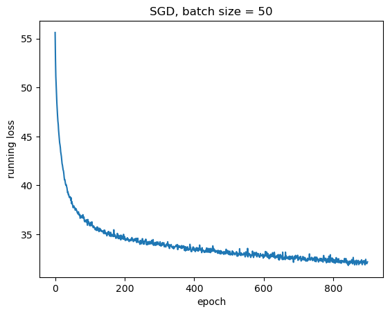
epochs = 900 # determined by hand to be around the best performance with given hyperparameters
loss_arr = [i for i in range(epochs)]
for epoch in range(epochs):
    running_loss = 0.0
    for i, data in enumerate(trainloader, 0):
        inputs, labels = data
        optimizer.zero_grad() # set optimizer to zero grad to remove previous epoch gradients
        outputs = clf(inputs) # forward propagation
        loss = criterion(outputs, labels)
        loss.backward() # backward propagation
        optimizer.step() # optimize
        running_loss += loss.item()
    # display statistics
    if epoch % 100 == 0:
        print(f'epoch: {epoch}, loss: {running_loss}')
    loss_arr[epoch] = running_loss

epoch: 0, loss: 55.62043100595474
epoch: 100, loss: 35.895830780267715
epoch: 200, loss: 34.766352623701096
epoch: 300, loss: 33.937689155340195
epoch: 400, loss: 33.5983669757843
epoch: 500, loss: 33.12820985913277
epoch: 600, loss: 32.83290234208107
epoch: 700, loss: 32.539843797683716
epoch: 800, loss: 32.337289214134216

plt.plot(loss_arr)
plt.xlabel("epoch")
plt.ylabel("running loss")
plt.title(f"SGD, batch size = {batch_size}")
plt.show()

Torch Testing

testdata = Data(X_test_np, y_test_np)
outputs = clf(testdata.X)
__, predicted = torch.max(outputs, 1)

print(accuracy_score(predicted,testdata.y))

0.7520547945205479

Accuracy around 76% is a decent score, considering random guess would generate 33% accuracy.

But can we make the Neural Network Model work better by selectively choosing the hyperparameters?

Finding Best Hyperparameter

Although the Torch neural network provides an example of how to handle a multi-layer perceptron, using scikit-learn’s MLPClassifier can accomplish this more efficiently. As the data set is relatively small, it can be processed quickly using a CPU. The focus of our inquiry is whether specific hyperparameters can consistently enhance the performance of this network. Essentially, our objective is to determine the level of predictive accuracy we can achieve by fine-tuning this neural network.

With much time testing out various hyper parameters, it turns out that “Simpler the Better”. Activation and Solver methods were generally more effective on “relu” and “adam”. As we reduce number of hidden layers and nuerons, the network tends to perform better. With much greater complexity, the network takes a longer time to train, and overfits the training data.

nn = MLPClassifier(hidden_layer_sizes = (10,10),
                   activation = "relu", # Activation function for the hidden layer.
                   solver='adam',
                   alpha = 0.001, # Strength of the L2 regularization term.
                   batch_size = 'auto',# Size of minibatches for stochastic optimizers.
                   learning_rate_init = 0.01, 
                   epsilon =1e-6,
                   max_iter = 1000,
                   shuffle = True,# shuffle samples in each iteration
                   early_stopping = True,
                   random_state=69,
                   verbose = False) # Allows to print progress messages to stdout.

nn.fit(X_train.values, y_train.values)

MLPClassifier(alpha=0.001, early_stopping=True, epsilon=1e-06,
              hidden_layer_sizes=(10, 10), learning_rate_init=0.01,
              max_iter=1000, random_state=69)

print(f"training score: {nn.score(X_train.values,y_train.values)}")
print(f"testing score: {nn.score(X_test.values,y_test.values)}")

training score: 0.7874493927125507
testing score: 0.7527397260273972

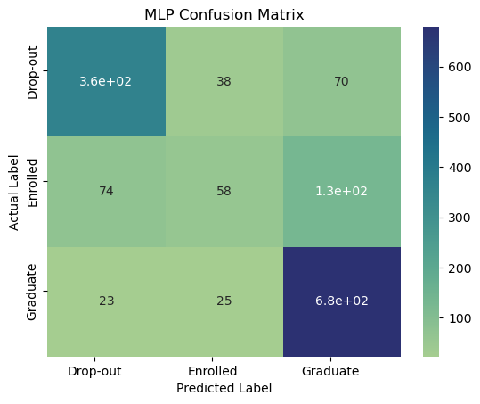
y_train_pred = nn.predict(X_test)
cnn_matrix = confusion_matrix(y_test,y_train_pred)
plot_confusion_matrix(cnn_matrix, title="MLP Confusion Matrix")

/Users/wonjoonchoi/opt/anaconda3/lib/python3.9/site-packages/sklearn/base.py:443: UserWarning: X has feature names, but MLPClassifier was fitted without feature names
  warnings.warn(

Comparing with Non-Neural Network ML

Although the neural network results are promising, they may not be entirely dependable in predicting dropout rates. Therefore, we need to generalize the question and ask if the reliability issue is related to the model type being used. To address this, we can compare the performance of the neural network with other machine learning models to determine which model produces the most reliable predictions.

Random Forest

When it comes to classification algorithms, data science offers a wide range of options such as logistic regression, support vector machine, naive Bayes classifier, and decision trees. However, one of the most powerful classifiers is the random forest classifier, which we will use for our investigation.

To build the RF model, we need to determine the ideal depth first.

# Finds best depth for Random Forest Classifier
def find_best_depth(model): 
    # Max Depth iteration
    N = 30
    # set initial list length of N
    scores = np.zeros(N)
    best_score = -np.inf
    
    for d in range(1,N+1):
                # set model with random state
        ref = model(max_depth=d,random_state=1111)
        # calculate score
        scores[d-1] = cross_val_score(ref,X_train,y_train,cv=5).mean() 
        if scores[d-1] >best_score:
                # update best_score and best_depth
                best_score=scores[d-1]
                best_depth = d
    
    # plot scatter plot
    fig, ax = plt.subplots(1) 
    ax.scatter(np.arange(1,N+1),scores)
    ax.set(title="Best Depth: " + str(best_depth)) 
    return best_depth

best_depth = find_best_depth(RandomForestClassifier)

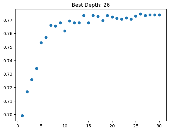
Knowing the best depth, we can now train the model

RF = RandomForestClassifier(max_depth=best_depth,random_state=1111)
RF.fit(X_train.values,y_train.values)

RandomForestClassifier(max_depth=26, random_state=1111)

RF.score(X_test.values,y_test.values)

0.760958904109589

We actually get a decent score, better than what we saw in NN

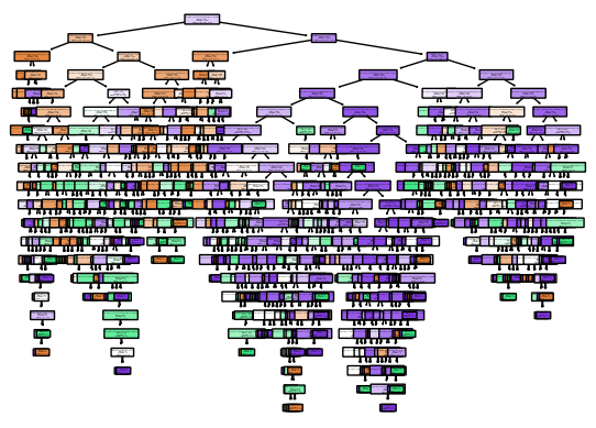
Lets Visualize what the model looks like

plot_tree(RF.estimators_[0], 
          feature_names= X_test.columns,
          class_names=["Drop out","Enrolled","Graduate"], 
          filled=True, impurity=True, 
          rounded=True)
plt.show()

y_train_pred = RF.predict(X_test.values)
RF_matrix = confusion_matrix(y_test.values,y_train_pred)
plot_confusion_matrix(RF_matrix, title="Random Forest Confusion Matrix")

Support Vector Machine

Now trying the SVM model

svm = SVC(kernel='linear')
svm.fit(X_train.values,y_train.values)
svm.score(X_test.values,y_test.values)

0.7465753424657534

y_train_pred = svm.predict(X_test)
svm_matrix = confusion_matrix(y_test,y_train_pred)
plot_confusion_matrix(svm_matrix, title="SVM Confusion Matrix")

/Users/wonjoonchoi/opt/anaconda3/lib/python3.9/site-packages/sklearn/base.py:443: UserWarning: X has feature names, but SVC was fitted without feature names
  warnings.warn(

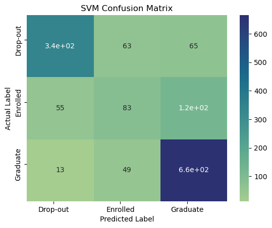
It’s possible that the data itself is limiting the accuracy of the models. Perhaps there are some variables that are missing or some variables that are not informative enough. It’s also possible that there are some complex interactions among the variables that the models are not capturing. Further investigation into the data and feature engineering may be necessary to improve the accuracy of the models. Additionally, it’s important to consider the practical implications of the models’ predictions and whether a slightly higher accuracy is worth the additional resources needed to achieve it.

Revisiting Preprocessing

As we revisit the initial stages of our analysis, there are a few questions we can address. First, how are we handling the categorical data in our models? Second, are there certain variables that have a higher impact on our prediction accuracy? Finally, can we standardize the data in any way to improve our results?

To explore these questions, we can experiment with different approaches and test their impact on the accuracy of our MLPClassifier neural network model. However, since changes to the input data may affect the hidden layer sizes, we will also use the Support Vector Classifier (SVC) as a standard benchmark for performance changes resulting from data processing.

One Hot Encoding

Treating categorical values as numerical values can lead to bias towards certain values and skew the results. Therefore, it’s more appropriate to represent each categorical variable as a binary vector using One Hot Encoding. This allows for unbiased representation of categorical data and ensures that each category is given equal weight in the analysis.

features.head()

	Marital status	Application mode	Application order	Course	Daytime/evening attendance	Previous qualification	Nationality	Mother's qualification	Father's qualification	Mother's occupation	...	Curricular units 1st sem (without evaluations)	Curricular units 2nd sem (credited)	Curricular units 2nd sem (enrolled)	Curricular units 2nd sem (evaluations)	Curricular units 2nd sem (approved)	Curricular units 2nd sem (grade)	Curricular units 2nd sem (without evaluations)	Unemployment rate	Inflation rate	GDP
0	1	8	5	2	1	1	1	13	10	6	...	0	0	0	0	0	0.000000	0	10.8	1.4	1.74
1	1	6	1	11	1	1	1	1	3	4	...	0	0	6	6	6	13.666667	0	13.9	-0.3	0.79
2	1	1	5	5	1	1	1	22	27	10	...	0	0	6	0	0	0.000000	0	10.8	1.4	1.74
3	1	8	2	15	1	1	1	23	27	6	...	0	0	6	10	5	12.400000	0	9.4	-0.8	-3.12
4	2	12	1	3	0	1	1	22	28	10	...	0	0	6	6	6	13.000000	0	13.9	-0.3	0.79

5 rows × 34 columns

categorical_labels = ['Marital status', 'Application mode', 'Application order', 'Course',
       'Daytime/evening attendance', 'Nationality',
       'Mother\'s occupation', 'Father\'s occupation', 'Displaced',
       'Educational special needs', 'Debtor', 'Tuition fees up to date',
       'Gender', 'Scholarship holder']

one_hot = pd.get_dummies(features,columns=categorical_labels)
one_hot.columns
X_train, X_test, y_train, y_test = train_test_split(one_hot, target, test_size=0.33)

nn = MLPClassifier(hidden_layer_sizes = (164,128,96), early_stopping = True) 

nn.fit(X_train.values, y_train.values)
print(f"training score: {nn.score(X_train.values,y_train.values)}")
print(f"testing score: {nn.score(X_test.values,y_test.values)}")

training score: 0.8454790823211876
testing score: 0.7636986301369864

clf = SVC(kernel='linear')
clf.fit(X_train.values,y_train.values)
clf.score(X_test.values,y_test.values)

0.7705479452054794

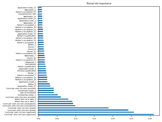
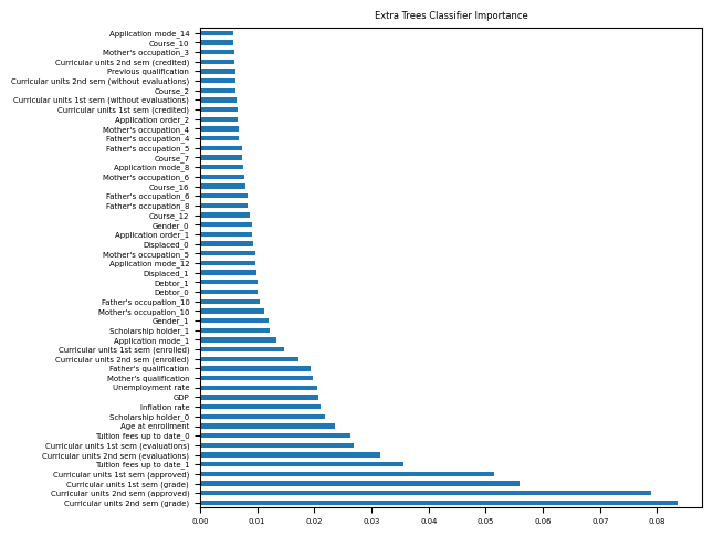
Feature Selection

In the process of One Hot Encoding, we split categorical variables into multiple columns which might introduce irrelevant data, leading to noise in the dataset.

In order to mitigate this, we can perform feature selection, which involves assessing the correlation of each column’s mutual information with the target variable or using decision trees to test the impact of variables on the target.

It’s important to note that feature selection is not the same as Principal Component Analysis (PCA), which only looks at features, whereas these methods also consider the target variable.

# feature selection
def select_features(features, target, num_features = 5, run_type = 0):
    plt.rcParams.update({'font.size': 5})
    if run_type == 0:
        importance = mutual_info_classif(features,target)
        ft_imp = pd.Series(importance, index=features.columns)
        title = "Mutual Info Importance"
    elif run_type == 1:
        model = ExtraTreesClassifier()
        model.fit(features,target)
        ft_imp = pd.Series(model.feature_importances_, index=features.columns)
        title = "Extra Trees Classifier Importance"
    
    largest = ft_imp.nlargest(num_features).index
    ft_imp.nlargest(num_features).plot(kind="barh")
    plt.title(title)
    plt.tight_layout()
    plt.show()

    return largest

largest = select_features(one_hot, target, 50, 0)

categorical_labels_filter = list(set(categorical_labels).intersection(largest))
X_train, X_test, y_train, y_test = train_test_split(one_hot[largest], target, test_size=0.33)

nn = MLPClassifier(hidden_layer_sizes = (50,40), early_stopping = True) 

nn.fit(X_train.values, y_train.values)
print(f"training score: {nn.score(X_train.values,y_train.values)}")
print(f"testing score: {nn.score(X_test.values,y_test.values)}")

training score: 0.7341430499325237
testing score: 0.7273972602739726

clf = SVC(kernel='linear')
clf.fit(X_train.values,y_train.values)
clf.score(X_test.values,y_test.values)

0.7698630136986301

largest = select_features(one_hot, target, 50, 1)
categorical_labels_filter = list(set(categorical_labels).intersection(largest))
X_train, X_test, y_train, y_test = train_test_split(
  one_hot[largest], target, test_size=0.33)

nn.fit(X_train.values, y_train.values)
print(f"training score: {nn.score(X_train.values,y_train.values)}")
print(f"testing score: {nn.score(X_test.values,y_test.values)}")

training score: 0.786774628879892
testing score: 0.7417808219178083

clf = SVC(kernel='linear')
clf.fit(X_train.values,y_train.values)
clf.score(X_test.values,y_test.values)

0.760958904109589

Data Standardization

Data features can have different ranges of values, which may create a bias towards certain features during the training process. This is especially problematic when using mathematical models. Standardization is a technique to address this issue, and involves shifting each feature to a comparable scale. StandardScaler is a specific method used for standardization that centers all features at zero and sets the standard deviation to one.

scaler = preprocessing.StandardScaler()
scaled_one_hot = one_hot.copy()
scale_features = features.columns.difference(categorical_labels)
for feature in scale_features:
    df_scaled = scaler.fit_transform(one_hot[feature].to_numpy().reshape(-1,1))
    scaled_one_hot[feature] = df_scaled
    
scaled_one_hot.head()

	Previous qualification	Mother's qualification	Father's qualification	Age at enrollment	International	Curricular units 1st sem (credited)	Curricular units 1st sem (enrolled)	Curricular units 1st sem (evaluations)	Curricular units 1st sem (approved)	Curricular units 1st sem (grade)	...	Educational special needs_0	Educational special needs_1	Debtor_0	Debtor_1	Tuition fees up to date_0	Tuition fees up to date_1	Gender_0	Gender_1	Scholarship holder_0	Scholarship holder_1
0	-0.386404	0.075111	-0.584526	-0.430363	-0.159682	-0.300813	-2.528560	-1.986068	-1.521257	-2.197102	...	1	0	1	0	0	1	0	1	1	0
1	-0.386404	-1.254495	-1.218380	-0.562168	-0.159682	-0.300813	-0.109105	-0.550192	0.418050	0.693599	...	1	0	1	0	1	0	0	1	1	0
2	-0.386404	1.072315	0.954834	-0.562168	-0.159682	-0.300813	-0.109105	-1.986068	-1.521257	-2.197102	...	1	0	1	0	1	0	0	1	1	0
3	-0.386404	1.183116	0.954834	-0.430363	-0.159682	-0.300813	-0.109105	-0.071567	0.418050	0.575611	...	1	0	1	0	0	1	1	0	1	0
4	-0.386404	1.072315	1.045384	2.864765	-0.159682	-0.300813	-0.109105	0.167746	0.094832	0.349468	...	1	0	1	0	0	1	1	0	1	0

5 rows × 182 columns

X_train, X_test, y_train, y_test = train_test_split(scaled_one_hot[largest], target, test_size=0.33)

nn = MLPClassifier(hidden_layer_sizes = (36,30,28), early_stopping = True) 

nn.fit(X_train.values, y_train.values)
print(f"training score: {nn.score(X_train.values,y_train.values)}")
print(f"testing score: {nn.score(X_test.values,y_test.values)}")

training score: 0.8238866396761133
testing score: 0.763013698630137

clf = SVC(kernel='linear')
clf.fit(X_train.values,y_train.values)
clf.score(X_test.values,y_test.values)

0.7678082191780822

After applying these preprocessing changes, the neural network’s performance has increased, compared to its initial performance. Although this improvement may not be the largest, it highlights how adjusting the fundamental features that are fed into a neural network can enhance its accuracy and reliability.

Conclusions

In conclusion, our analysis has allowed us to identify certain traits that can help predict students at higher risk of dropping out of college. By recognizing these early warning signs, we can allocate resources and attention to those in need to help prevent them from dropping out.

However, our exploration of using neural networks for this task did not yield better results compared to other machine learning methods. Despite trying different model structures, activation functions, solvers, one-hot encoding, and pre-processing techniques, neural networks did not show significant improvements in classifying the data.

The limitations of our study can be attributed to the sparsity of the data, the limited sample size, and the possibility of not finding the optimal hyperparameters for the neural network. Therefore, it may not be ideal to use neural networks for classification problems in cases where the data is too sparse or the sample size is limited.

Overall, while our results provide valuable insights into predicting dropout rates, more research is needed to explore the potential of neural networks in educational data mining and learning analytics.

Future Directions

Our analysis has identified that both neural networks and other machine learning methods struggled with predicting the “Enrolled” status, while accurately predicting the “Drop-out” status is of greater importance to our study.

As a result, a potential future direction could be to modify the classification task to focus solely on predicting the likelihood of “Drop-out” and evaluate the performance of the models in this context. This approach may help improve the performance of the models, and it would be interesting to investigate whether different machine learning methods would exhibit different levels of improvement in predicting “Drop-out” status.

Furthermore, future research could focus on addressing the limitations of our study by acquiring more comprehensive and diverse data sets, employing more sophisticated feature engineering and selection techniques, and exploring alternative modeling strategies to improve the predictive power of the models.

Sources

Realinho, V.; Machado, J.; Baptista, L.; Martins, M.V. Predicting Student Dropout and Academic Success. Data 2022, 7, 146. https://doi.org/10.3390/data711014

College graduates statistics. ThinkImpact.com. (2021, September 22). Retrieved March 19, 2023, from https://www.thinkimpact.com/college-graduates-statistics/